Overview
Use the Intel® Distribution of OpenVINO™ toolkit to detect brain tumors in MRI images. A U-Net topology-based pretrained model from open source datasets helps predict results and compare accuracy with provided ground truth results using the Sørensen–Dice coefficient.
Select Configure & Download to download the reference implementation and the software listed below.
To run this sample application as an interactive Jupyter* Notebook in Intel® Developer Cloud for the Edge with a bare metal infrastructure, select Launch Now. Intel Developer Cloud for the Edge is a free resource for prototyping, benchmarking performance, and testing AI solutions.
- Time to Complete: Approximately 30-40 minutes
- Programming Language: Python*
- Available Software: Intel® Distribution of OpenVINO™ toolkit 2021.4
Recommended Hardware
The hardware below is recommended for use with this reference implementation. For other suggestions, see Recommended Hardware.
Target System Requirements
- 6th to 11th Generation Intel® Core™ processors with Intel® Iris® Plus Graphics or Intel® HD Graphics
- Disk space needed: 20 GB
- RAM usage by application: 1.5 – 2 GB
- Ubuntu* 20.04 LTS
NOTE: We recommend that you use a 4.14+ Linux* kernel with this software. Run the following command to determine your kernel version: uname -a
How It Works
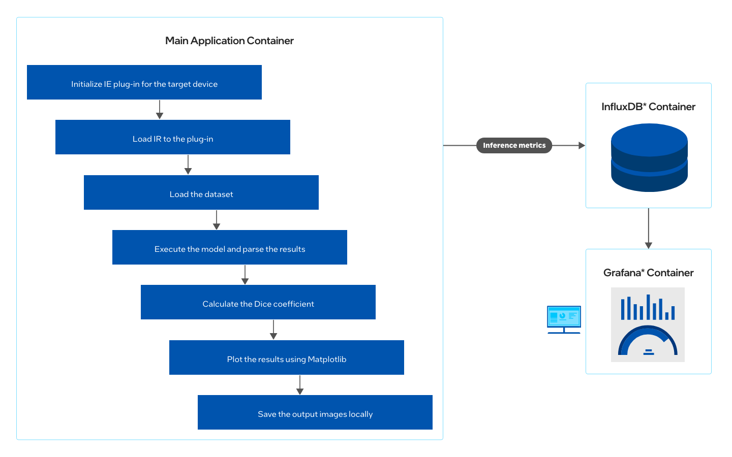
Using a combination of different computer vision techniques, this reference implementation performs brain tumor image segmentation on MRI scans, compares the accuracy with ground truth using Sørensen–Dice coefficient, and plots the performance comparison between TensorFlow* and OpenVINO™ optimized model.
- Train the model using an open source dataset from the Medical Segmentation Decathlon for segmenting brain tumors in MRI scans. More Information.
- Optimize the model using OpenVINO™ optimizer.
- Use the optimized model with the inference engine to predict results and compare accuracy with provided ground truth results using the Sørensen–Dice coefficient.
- Plot the performance comparison between TensorFlow* and OpenVINO™ optimized model.
- Store the output images from the segmented brain tumor locally.
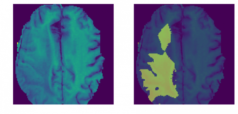
The Dice coefficient (the standard metric for the BraTS dataset used in the application) for this model is about 0.82-0.88. Menze et al. reported that expert neuroradiologists manually segmented these tumors with a cross-rater Dice score of 0.75-0.85, meaning that the model’s predictions are on par with what expert physicians have made. The below MRI brain scans highlight brain tumor matter segmented using deep learning.
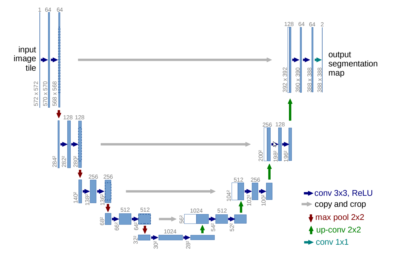
The U-Net architecture is used to create deep learning models for segmenting nerves in ultrasound images, lungs in CT scans, and even interference in radio telescopes.
U-Net is designed like an auto-encoder. It has an encoding path (“contracting”) paired with a decoding path (“expanding”) which gives it the “U” shape. However, in contrast to the auto-encoder, U-Net predicts a pixelwise segmentation map of the input image rather than classifying the input image as a whole. For each pixel in the original image, it asks the question: “To which class does this pixel belong?” This flexibility allows U-Net to predict different parts of the tumor simultaneously.
Get Started
Prerequisites
- Ensure that InfluxDB* and Grafana* services are not running on your system. The ports 8086 and 3000 must be free. The application will not run if ports are occupied.
- Ensure that at least 20 GB of storage and 2 GB of free RAM space are available on the system.
- Ensure that internet is available on the system. (Set proxies if running on a proxy network.)
Which model to use
The application uses a pre-trained model (saved_model_frozen.pb), that is provided in the /resources directory in GitHub.
This model is trained using the Task01_BrainTumour.tar dataset from the Medical Segmentation Decathlon, made available under the (CC BY-SA 4.0) license. Instructions on how to train your model can be found on GitHub.
What input to use
The application uses MRI scans from Task01_BrainTumour.h5 (a subset of 8 images from the BraTS dataset taken at random), that is provided in the /resources directory in GitHub.
NOTE: You can also provide your own patient data file (in nii.gz format) from the BraTS dataset and run the application to see the inference. See Provide User Specific Data for Inference.
Step 1: Install the Reference Implementation
Select Configure & Download to download the reference implementation and then follow the steps below to install it.
- Open a new terminal, go to the downloaded folder and unzip the RI package.
unzip brain_tumor_segmentation.zip - Go to the brain_tumor_segmentation directory.
cd brain_tumor_segmentation - Change permission of the executable edgesoftware file.
chmod 755 edgesoftware - Run the command below to install the reference implementation:
./edgesoftware install - During the installation, you will be prompted for the Product Key. The Product Key is contained in the email you received from Intel confirming your download.
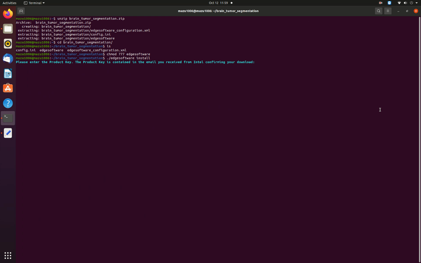
Figure 4. Installation Start
- When the installation is complete, you see the message Installation of package complete and the installation status for each module.
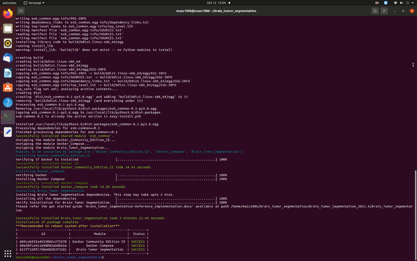
Figure 5. Installation Success
Step 2: Run the Reference Implementation
- Enter the following command to see the application containers successfully created and running:
You will see output similar to:docker ps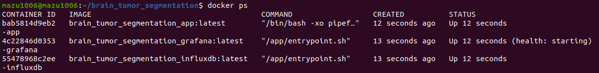
Figure 6. List of Containers
- To visualize the data and dashboards on Grafana and InfluxDB, follow the steps below.
- From the brain-tumor-segmentation folder path, execute the commands:
sudo docker-compose down
sudo docker volume prune
- Open the .env file in the same folder path with your preferred editor and edit the following parameters. The example below uses vim.
vim .env
Under Grafana Options:GF_SECURITY_ADMIN_USER=admin GF_SECURITY_ADMIN_PASSWORD=admin
Under Influx Options:# To generate an Admin Token $ openssl rand -hex 32 # Username, Password, Org Name, Bucket (Database Name) DOCKER_INFLUXDB_INIT_USERNAME=admin DOCKER_INFLUXDB_INIT_PASSWORD=password123 DOCKER_INFLUXDB_INIT_ADMIN_TOKEN=<generated-token> DOCKER_INFLUXDB_INIT_ORG=intel DOCKER_INFLUXDB_INIT_BUCKET=Brain_Tumor_Segmentation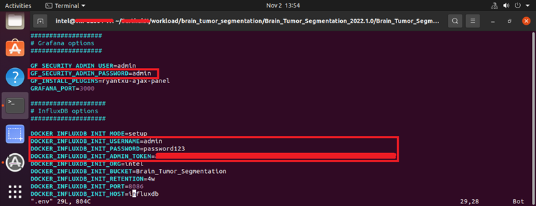
Figure 7: .env File Parameters
-
Bring up the application containers by executing the command:
sudo docker-compose up -d
- From the brain-tumor-segmentation folder path, execute the commands:
- Once the application containers are up successfully, open the Grafana dashboard by visiting http://localhost:3000/ on your browser. Enter username and password as admin.
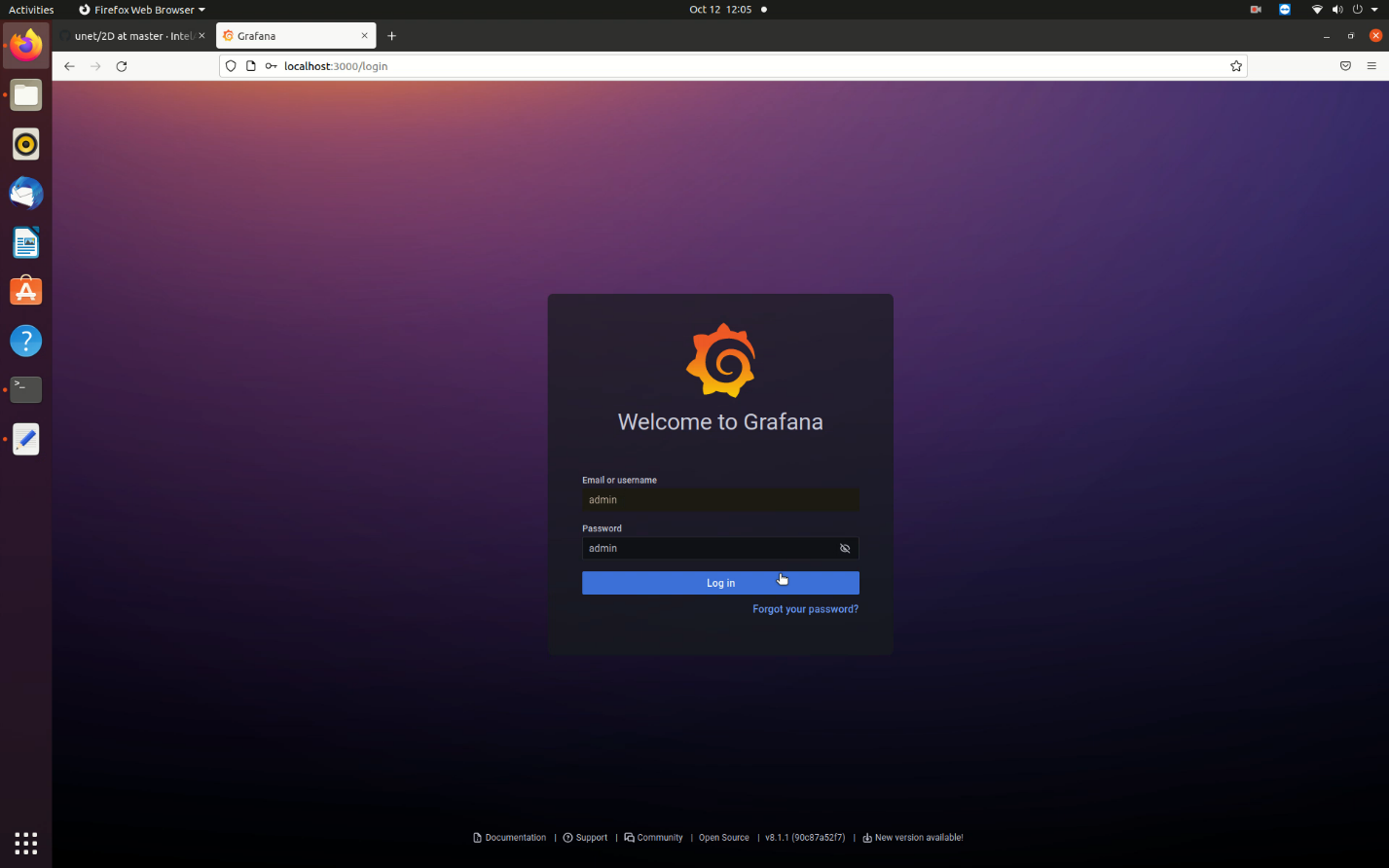
Figure 8. Grafana Login Screen
- Go to the Dashboards menu and click on Manage. The list of available dashboards is shown. In this case, only the Brain Tumor Segmentation dashboard is available.
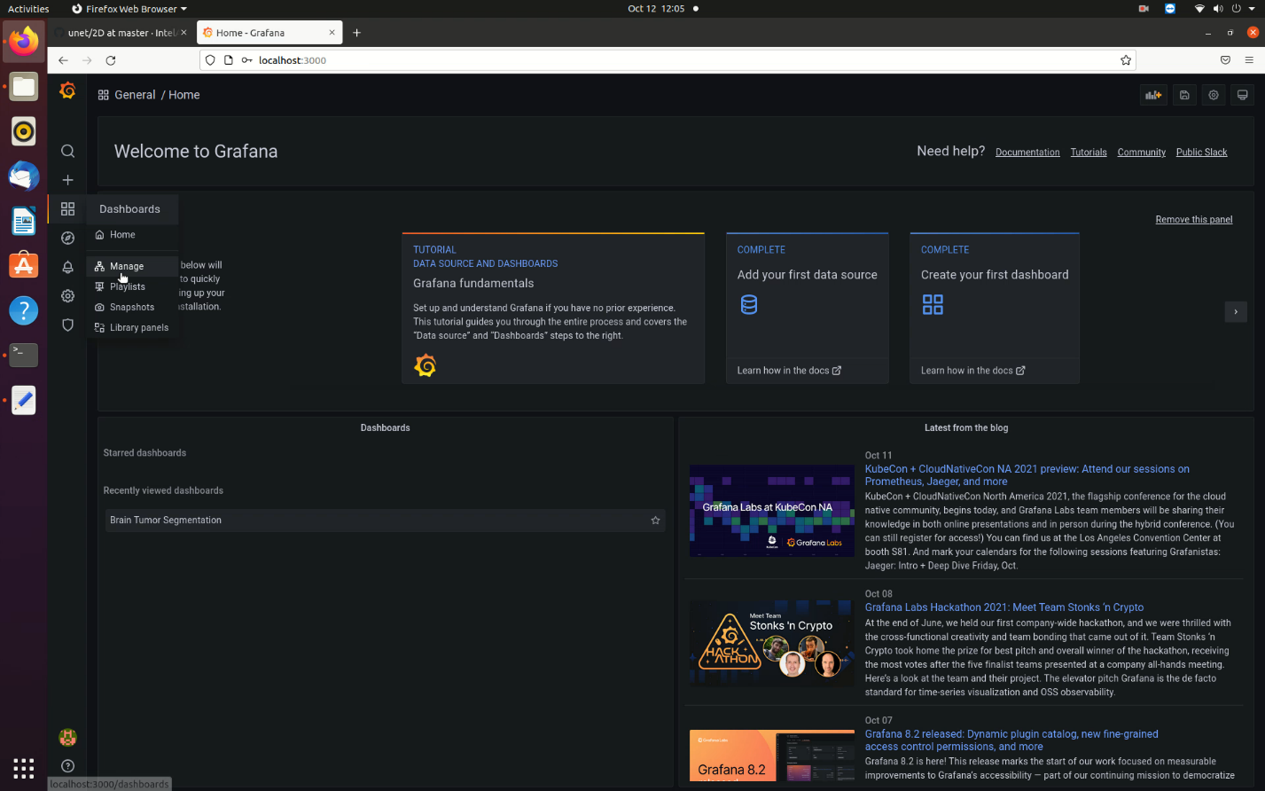
Figure 9. Manage Dashboards in Grafana
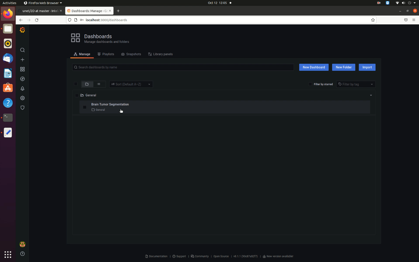
Figure 10. List of Available Dashboards
- Open the Brain Tumor Segmentation dashboard to view the inferenced images and the comparison metrics between the OpenVINO™ toolkit and TensorFlow inference.
Ensure you select the refresh every 5s option to view the live dashboard as shown in the image below.
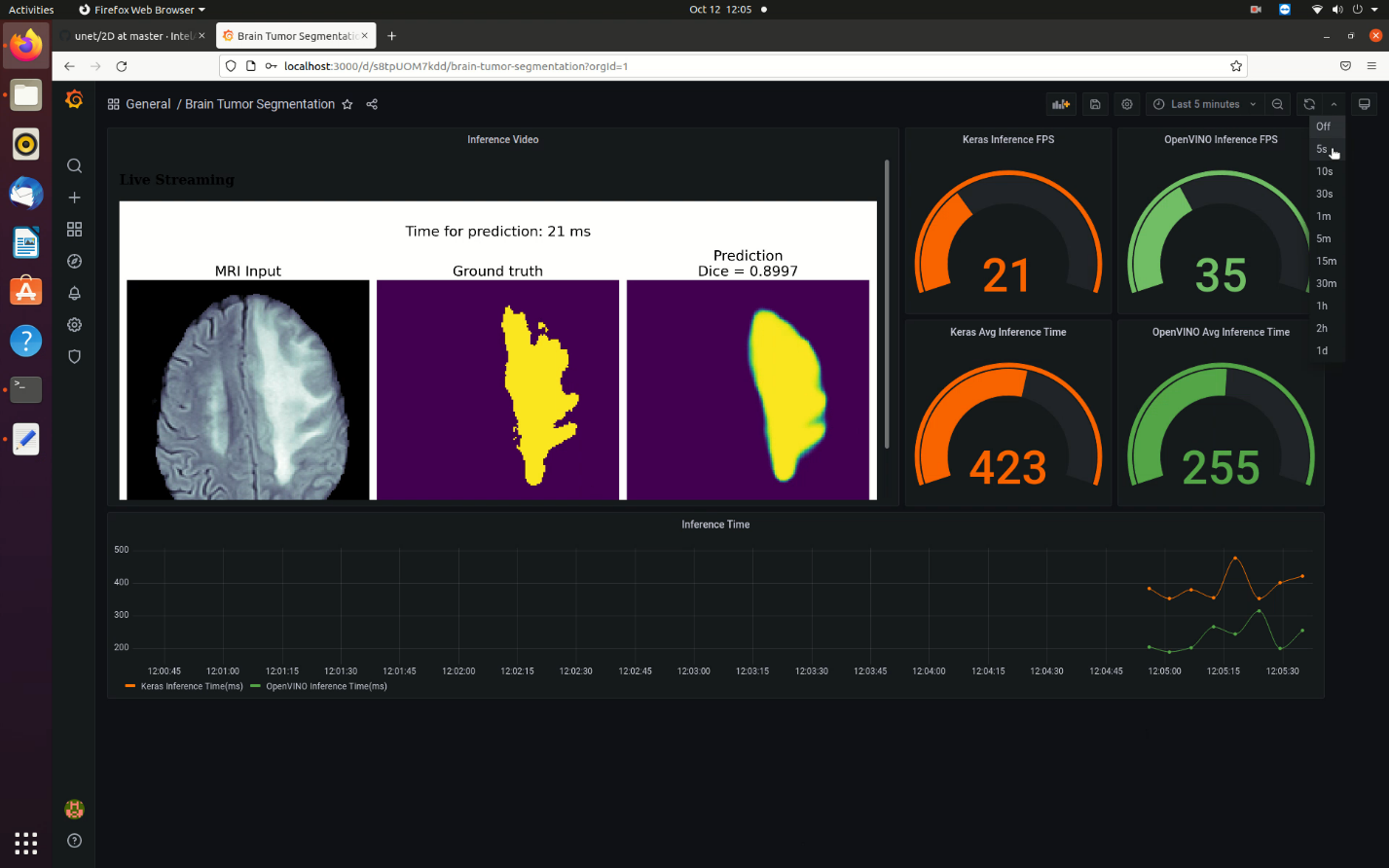
Figure 11. Brain Tumor Segmentation Dashboard
The Grafana dashboard shows the following noteworthy items:- The image in the dashboard shows the MRI scan (left), the ground truth marked by medical experts [also known as the mask] (center) and prediction by the u-net model (right). There is also the time taken for inference by OpenVINO™ toolkit (per image) on the top and the DICE score to estimate accuracy of inference against the ground truth.
- The circular gauges on the top-right indicate the comparison between the FPS rates of inference by OpenVINO™ toolkit and TensorFlow.
- The circular gauges on the mid-right indicate the comparison between the avergage inference time (in ms) by OpenVINO™ toolkit and TensorFlow for the complete set of images (one iteration).
- The timeseries chart (bottom) shows the live time taken for inference (in ms) comparison between OpenVINO™ toolkit and TensorFlow.
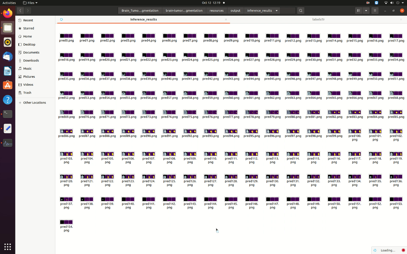
- To view the inference images, go to the installation directory and then to the location shown below:
<installation_directory>/brain_tumor_segmentation/Brain_Tumor_Segmentation_2021.4/Brain_Tumor_Segmentation/brain-tumor-segmentation/resources/output/inference_results/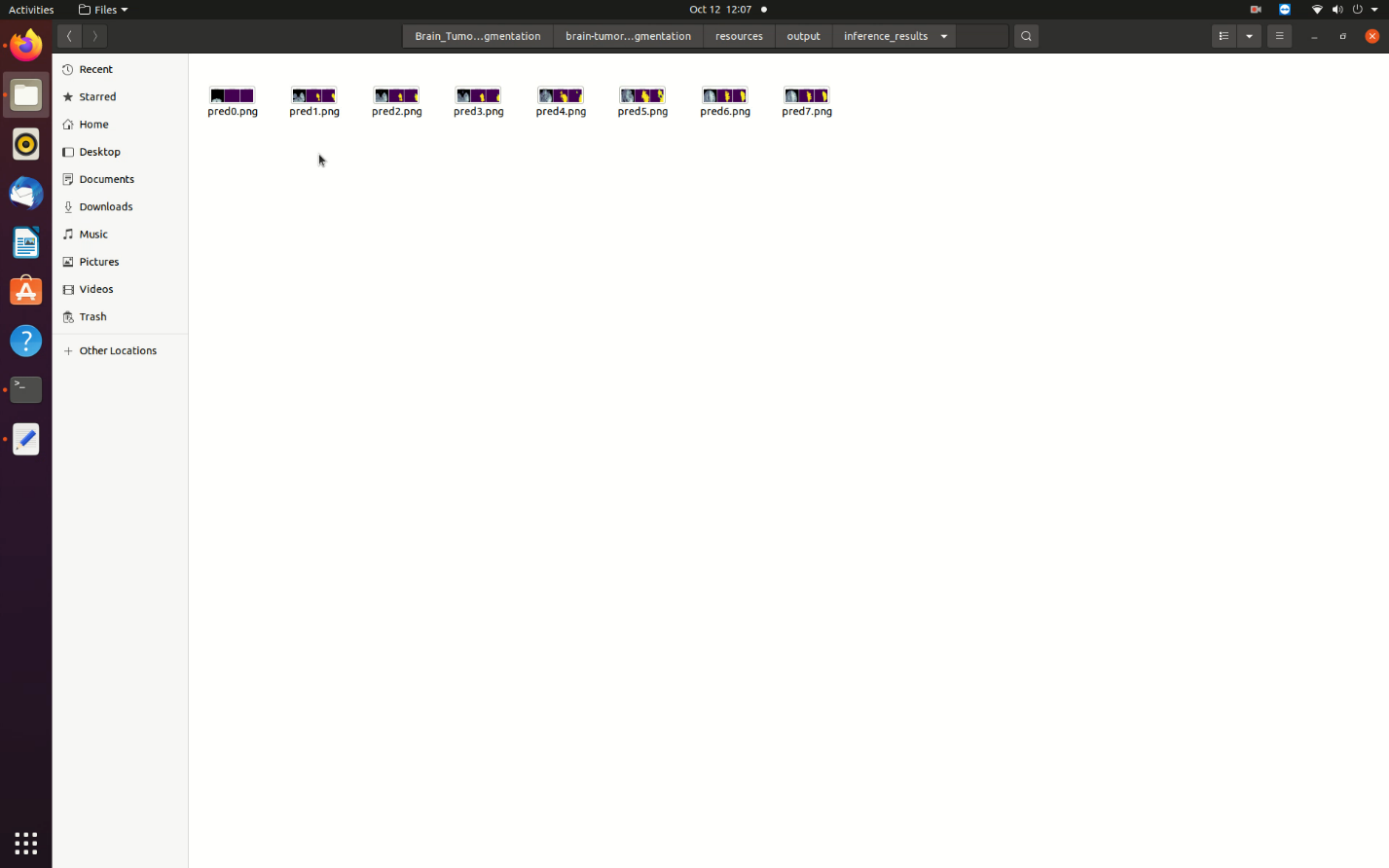
Figure 12. Saved Images Folder
- Similarly, to view the InfluxDB dashboard, go to http://localhost:8086 on your browser. Log in with username as admin and password as password123. To view the dashboards, select Explore from the left hand side pane of the InfluxDB UI and select the options you require.
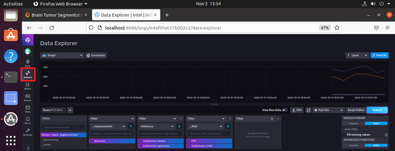
Figure 13: InfluxDB Dashboard
Configure the Reference Implementation
Open the config.json file located in the resources folder:
<installation_directory>/brain_tumor_segmentation/Brain_Tumor_Segmentation_2021.4/Brain_Tumor_Segmentation/brain-tumor-segmentation/resources/
The file contents are various parameters that affect the operation of this application:
{
    "defaultdata": 1,
    "imagedatafile": "../resources/nii_images/MRIScans/BRATS_006.nii.gz",
    "maskdatafile": "../resources/nii_images/Masks/BRATS_006.nii.gz",
    "n_iter": 300,
    "maxqueuesize": 25,
    "targetdevice": "cpu",
    "saveimage": 1
}
Description of parameters:
- defaultdata: This parameter toggles the application to use either default data (1) or user specific data from BraTS dataset (0) for inference.
- imagedatafile: This parameter contains the path for the mri scan image data file when user specific data is provided (defaultdata = 0) in nii.gz format.
- maskdatafile: This parameter contains the path for the mask (ground truth) image data file when user specific data is provided (defaultdata = 0) in nii.gz format.
- n_iter: This parameter specifies the number of iterations the application must run the set of images to get a long running estimate of inference by OpenVINO™ toolkit and TensorFlow.
- maxqueuesize: Since Flask server is used to publish images into Grafana, a queue implementation is in place to store images from which the server pushes into the port for viewing. This parameter controls the number of images in queue to reduce the RAM usage (since the queue uses volatile memory). In short, lower the number, lower the RAM usage; however, you may lose a few images since the program will discard images when the queue is full.
- targetdevice: This parameter helps select the target device (CPU/GPU/VPU, etc.) on which the inference must run.
- saveimage: This parameter when toggled OFF (0) disables the saving of images on local storage. ON (1) will store the inference images and overwrite the existing ones when the application is re-run.
Provide User Specific Data for Inference
- Ensure the defaultdata is set to ‘0’.
- Download the BraTS dataset.
- Extract the dataset and select any patient file number from the Imagestr and the labelstr folders. The Imagestr folder contains the MRI scans where each file (nii,gz format) has 155 brain MRI images of a single patient slice by slice. The labelstr folder contains the files for the ground truth of the 155 slices of scans.
- Ensure same patient file from Imagestr and labelstr are selected (BRATS_xxx.nii.gz).
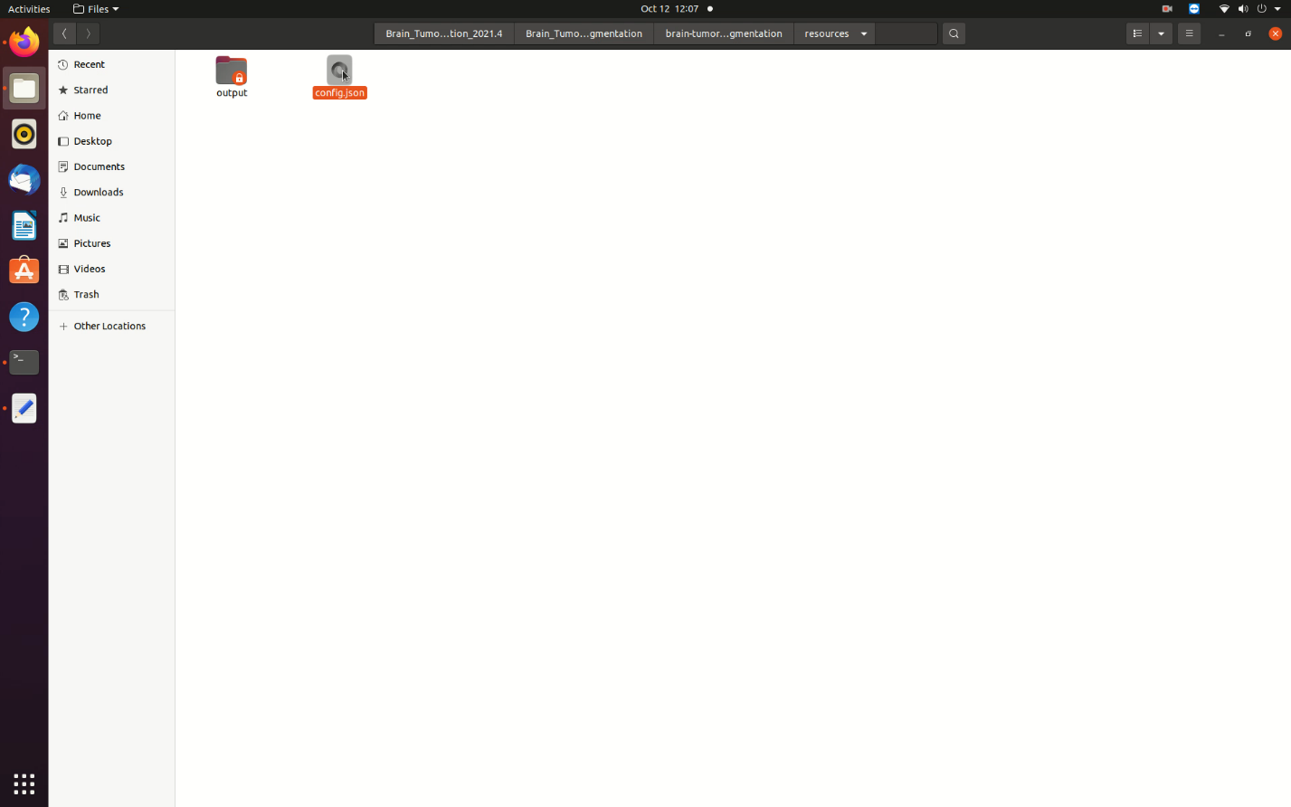
- Create a folder inside the resources folder to contain the user specific images. The example below uses user_image.
- Create two separate folders to contain the mri scan and mask file. (Any name is ok.) The example below uses mri_scan and mask.
- Enter the folder location and file name for the mri scan and mask in the config file as shown in the image below:
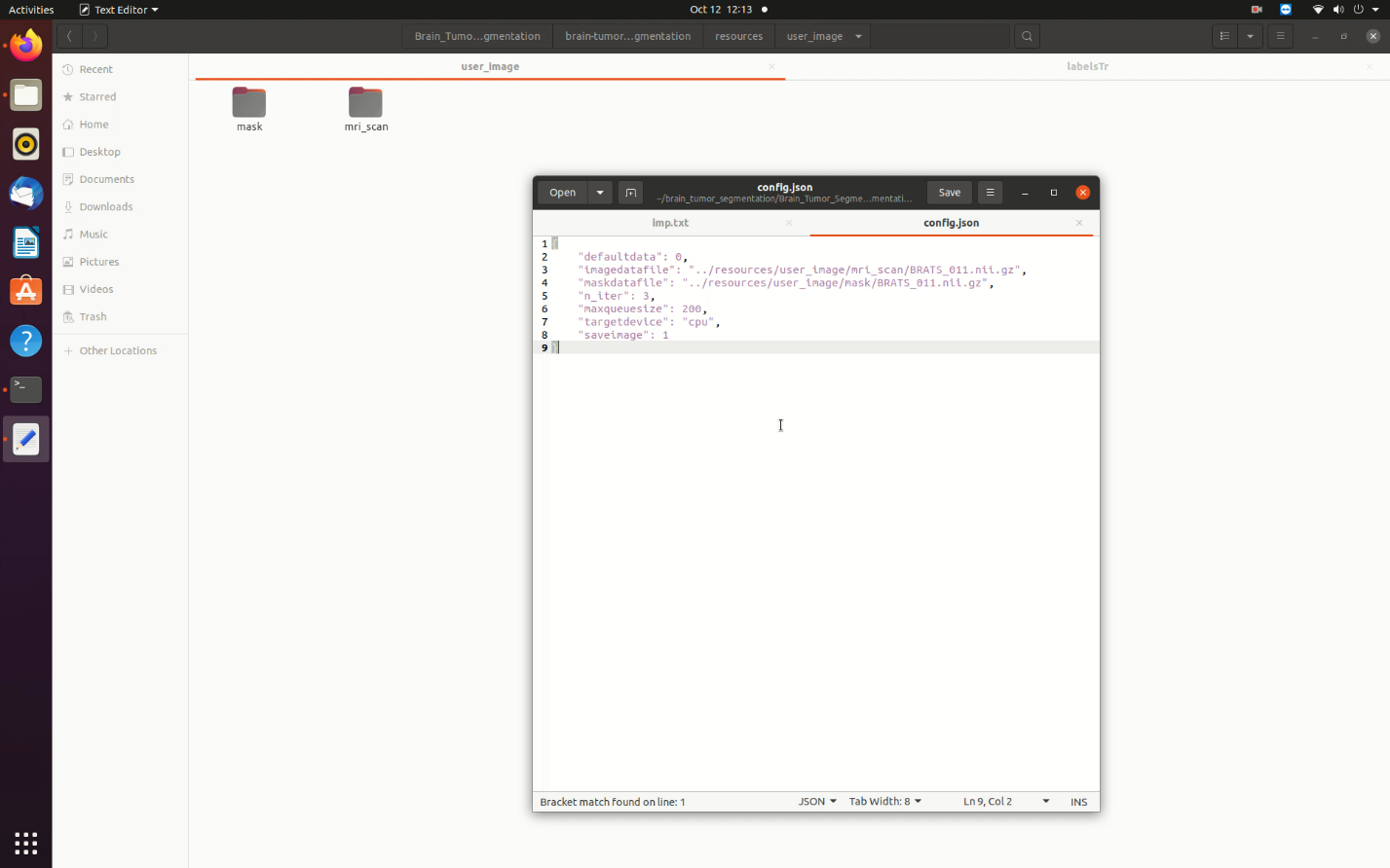
Figure 15. User Specific Images Configuration
- Save the config file and restart the Docker container by entering the following command:
The <container_id or name> value can be obtained from the docker ps command.docker restart <container_id or name>
The patient file contains 155 images and each iteration of the application will take more time to compute. After the first iteration, the inference images are stored in the inference_results folder (if saveimage = 1).
Summary and Next Steps
With this application you successfully used the Intel® Distribution of OpenVINO™ Toolkit to create a solution that detects brain tumors in MRI images.
As a next step, try going through the application code available in the app folder and add a post inference code to isolate the tumor and generate a 3D model for the tumor since this application runs the slice by slice 155 2D images of a single brain.
Learn More
To continue learning, see the following guides and software resources:
Troubleshooting
Known Issues
Installation Failure
The root cause can be analyzed by looking at the installation logs in the /var/log/esb-cli/Brain_Tumor_Segmentation_2021.4/Brain_Tumor_Segmentation/install.log file.
Unable to Run apt Install While Building Images
This issue occurs when proxy is configured for the network in use.
Solution: Set the proxy inside the containers too while they are built.
Add the below mentioned two lines in the top of the app dockerfile (<installation_directory>/brain_tumor_segmentation/Brain_Tumor_Segmentation_2021.4/Brain_Tumor_Segmentation/brain-tumor-segmentation/app/) and the Grafana dockerfile (<installation_directory>/brain_tumor_segmentation/Brain_Tumor_Segmentation_2021.4/Brain_Tumor_Segmentation/brain-tumor-segmentation/utils/grafana/) after the license information.
ENV HTTP_PROXY <your http proxy>
ENV HTTPS_PROXY <your https proxy>
Address Already in Use
If running the application results in Error starting userland proxy: listen tcp4 0.0.0.0:3000: bind: address already in use, use the following command to check and force stop the process:
sudo kill $(pgrep grafana)
NOTE: If the issue persists, it may be possible that Grafana is running in a Docker container. In that case, stop the container using:
sudo docker stop $(sudo docker ps -q --filter expose=3000)
If running the application results in Error starting userland proxy: listen tcp4 0.0.0.0:8086: bind: address already in use, use the following command to check and force stop the process:
sudo kill $(pgrep influxdb)
NOTE: If the issue persists, it may be possible that InfluxDB is running in a Docker container. In that case, stop the container using:
sudo docker stop $(sudo docker ps -q --filter expose=8086)
Grafana Dashboard Not Showing Image Sequence
This might happen due to internal Flask Server and Ajax panel compatibility issue. Run http://localhost:5000/ in another tab of the browser to view the image sequence.
File Not Found
This might happen due to incorrect file location of the image and mask data files in the config file. Recheck the folder path and ensure the location starts with ../resources/ since the code runs inside the app folder.
Config Parameter Errors
Config file parameters have very specific input requirements, which will be clearly explained in the logs as error messages.
Support Forum
If you're unable to resolve your issues, contact the Support Forum.